Another post inspired by questions on SE, see here or here. And great opportunity to explore tagging of bicycle related features in OpenStreetMap. An example based on Wrocław, medium size (680 000 inhabitants) town in south-west part of Poland.
Highways and tracks
In OpenStreetMap data the roads designated for bicycle can be described in different ways. The lanes can be separate, can be part of general highway, or shared with pedestrians (and in some countries even with other vehicles). Let’s have a quick overview of the used tags.
This is non exhaustive list of all possible tags which can be used. For more information see wiki description of cycleway and bicycle infrastructure.
Separate ways for cycling usually are described as highway = cycleway, and in the field they are marked with white bicycle on blue background sign.1
highway = cycleway
If the cycling lane is shared with pedestrians, the usual tagging is:
highway = footway | path
bicycle = designated
foot = designated

Another possibility is to share the lane with cars on any highway (primary, tertiary, residential, etc). It can be the lane in the same or opposite direction. Tagging
highway = *
cycleway = lane


is used to tag two-way streets where there are cycle lanes on both sides of the road, or one-way streets where the lane operating in the same direction as main traffic flow. cycleway = opposite_lane is used for contraflow; cycleway = opposite + oneway:bicycle = no where cyclist are permitted to travel in both direction on one-way street. For shared lanes with motor vehicles: cycleway = shared_lane and cycleway=share_busway with buses. For more specific tagging please check OpenStreetMap wiki page.
In some countries additional tagging is in use. highway = * + bicycle_road = yes for signed roads and cyclestreet = yes for roads where other vehicles are allowed.2

Other features
Bicycle shops are tagged with shop = bicycle, and those which provide additional repair services have service:bicycle:pair = yes tags. There might be a do-it-yourself service stations, equipped with pump, wrenches and other helpful tools — in such case they are tagged with amenity = bicycle_repair_station.
Bicycle parkings are tagged with amenity = bicycle_parking. In towns where you can rent a bike, you will find amenity = bicycle_rental tags.
Bicycle routes
Cycle routes or bicycle route are named or numbered or otherwise signed routes. May go along roads, trails or dedicated cycle paths.3
They are tagged as a relations (several features grouped together with relation roles assigned)4; they can be of different network levels: network = icn | ncn | rcn | lcn which corresponds to international route, a national route, a regional route or a local route. Below an example of tagging of Polish part of EuroVelo 9 route, which crosses Wrocław:
type = route
route = bicycle
network = icn
ref = EV9
colour = green
icn_ref = 9
As we already know and understand the attributes of the data, let’s play with it a bit. In next paragraph we will assess quantitatively the bicycle infrastructure in Wrocław.
Wrocław’s infrastructure
For data access/download we will use osmdata package (Padgham et al. 2017, 2022). We will download town boundary, highways and other bicycle infrastructure. We will save the data for further reuse.
Code
get_osm_data <- function(place, feature, output_dir = "data") {
  output_dir = paste0({{output_dir}}, "/", iconv(place, to="ASCII//TRANSLIT"))
  if(!dir.exists(output_dir)) dir.create(output_dir, recursive = TRUE)
  data_file = paste0(output_dir, "/", feature, ".rds")
  if(!file.exists(data_file)) {

    bb <- osmdata::getbb(place, featuretype = "city")
    switch(feature,
           boundary = {
             message(paste("Downloading boundary for", place))
             osm_data <-osmdata::opq(bb, timeout = 25*100) |>
               osmdata::add_osm_feature(key = "boundary", value = "administrative") |>
               osmdata::add_osm_feature(key = "admin_level", value = "6") |>
               osmdata::osmdata_sf() |>
               osmdata::unique_osmdata()
             saveRDS(osm_data, file = data_file)
           },
           highway = {
             message(paste("Downloading highways for", place))
             osm_data <-osmdata::opq(bb, timeout = 25*100) |>
               osmdata::add_osm_features(features = c("\"highway\"", "\"cycleway\"")) |>
               osmdata::osmdata_sf() |>
               osmdata::unique_osmdata()
             saveRDS(osm_data, file = data_file)
           },
           bicycle = {
             message(paste("Downloading bicycle infrastructure for", place))
             osm_data <-osmdata::opq(bb, timeout = 25*100) |>
               osmdata::add_osm_feature(key = "bicycle") |>
               osmdata::osmdata_sf() |>
               osmdata::unique_osmdata()
             saveRDS(osm_data, file = data_file)
           }
        )
  } else {
    message(paste("File", data_file, "already exists"))
  }
}

features <- list("boundary", "highway", "bicycle")
lapply(seq_along(features), function(i) get_osm_data("Wrocław", features[[i]], output_dir = "data"))
Having the data downloaded we can start our analysis. As first step we will create Wrocław’s boundary as sf polygon, it will be used to crop remaining data sets to city limits.
tb <- readRDS("data/Wroclaw/boundary.rds")
tb <- tb$osm_multipolygons |>
  subset(name == "Wrocław") |>
  subset(select = c("name", "geometry")) |>
  sf::st_as_sf()
sf::write_sf(tb, dsn = "data/wroclaw.gpkg", layer = "boundary", delete_layer = TRUE)
Highways and cycleways. As they might be returned from Overpass query as osm_lines and osm_multilines we have to bind them together.
highways <- readRDS("data/Wroclaw/highway.rds")
  hw <- highways$osm_lines |>
    dplyr::select("osm_id", "name", "highway", "bicycle",
                  "foot", starts_with(c("cycleway")), "oneway",
                  "surface", "vehicle")
  if(!is.null(highways$osm_multilines)) {
    multilines <- highways$osm_multilines |>
      dplyr::select("osm_id", "name", "highway", "bicycle",
                    "foot", starts_with(c("cycleway")), "oneway",
                    "surface", "vehicle")
    hw <- rbind(hw, multilines) |>
      sf::st_as_sf()
  }
hw <- suppressWarnings(sf::st_intersection(hw, tb))
sf::write_sf(hw, dsn = "data/wroclaw.gpkg", layer = "highways", delete_layer = TRUE)
With the highways prepared, let’s run simple analysis: count the length of the roads for bikes, bikes + pedestrians, and cars only.
Bike only
ddr <- hw |>
  dplyr::filter(highway == "cycleway" | cycleway %in% c("lane", "track", "yes")) |>
  dplyr::summarise(geometry = sf::st_union(geometry)) |>
  dplyr::mutate(length = units::set_units(sf::st_length(geometry), "km")) |>
  dplyr::mutate(category = "Bikes only") |>
  sf::st_drop_geometry()
Very similar approach for other categories.
Code
ddrip <- hw |>
  dplyr::filter(highway %in% c("path", "footway")) |>
  dplyr::filter(bicycle == "designated") |>
  dplyr::summarise(geometry = sf::st_union(geometry)) |>
  dplyr::mutate(length = units::set_units(sf::st_length(geometry), "km")) |>
  dplyr::mutate(category = "Bikes + Pedestrians") |>
  sf::st_drop_geometry()

cars_only <- hw |>
  dplyr::filter(!highway %in% c("cycleway", "path", "footway")) |>
  dplyr::filter(is.na(cycleway.left) | is.na(cycleway.right)) |>
  dplyr::summarise(geometry = sf::st_union(geometry)) |>
  dplyr::mutate(length = units::set_units(sf::st_length(geometry), "km")) |>
  dplyr::mutate(category = "Cars only") |>
  sf::st_drop_geometry()

#' and let's bind them together

ddr |>
  rbind(ddrip) |>
  rbind(cars_only) |>
  dplyr::mutate(l = "Total length") |>
  tidyr::pivot_wider(names_from = category, values_from = length) |>
  dplyr::mutate(across(2:4, ~format(round(.x, 1), nsmall = 1))) |>
  kableExtra::kbl(booktabs = TRUE, escape = F, linesep = "",
    col.names = kableExtra::linebreak(c("", "Bikes only", "Bikes + Pedestrians", "Cars only"), align = "c"),
    align = c("crrr")) |>
kableExtra::kable_styling()| Bikes only | Bikes + Pedestrians | Cars only | |
|---|---|---|---|
| Total length | 135.7 [km] | 213.9 [km] | 3717.6 [km] |
Not much, as for 680k inhabitants town, around 0.5 km per 1000 ppl. And less than 10% in comparison to cars road network…
If you would like to split it by surface (asphalt, concrete, etc), then we can just group our highways by that column, like
ddr <- hw |>
  dplyr::filter(highway == "cycleway" | cycleway %in% c("lane", "track", "yes")) |>
  dplyr::group_by(surface) |>
  dplyr::summarise(geometry = sf::st_union(geometry)) |>
  [...]
Which gives:
| Surface | Length [km] |
|---|---|
| asphalt | 96.14 |
| paving_stones | 23.66 |
| NA | 12.76 |
| paved | 0.91 |
| concrete | 0.76 |
| sett | 0.73 |
| unpaved | 0.24 |
| compacted | 0.23 |
| dirt | 0.18 |
| concrete:plates | 0.06 |
| fine_gravel | 0.03 |
| metal | 0.01 |
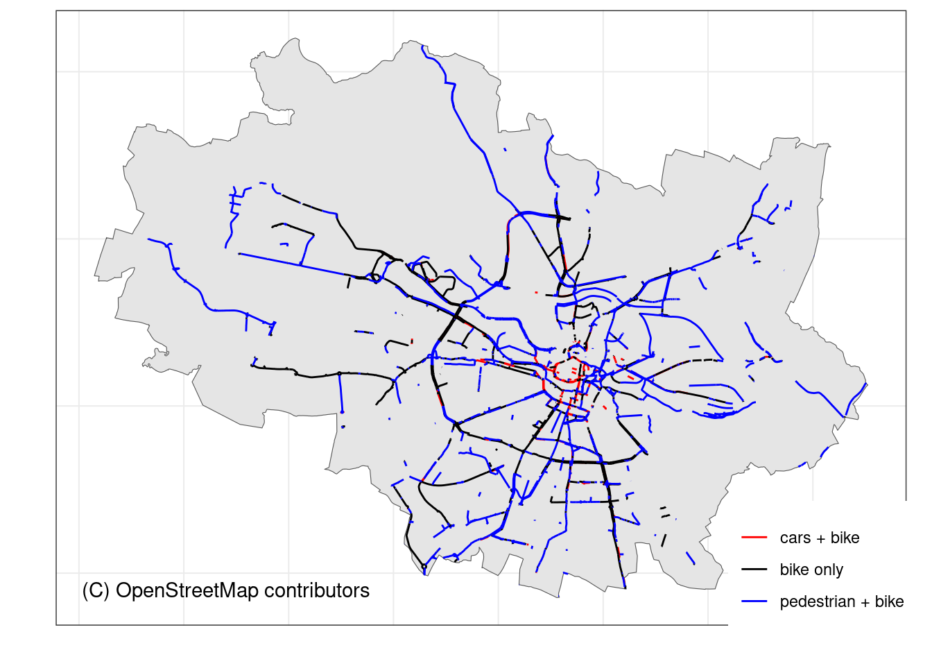
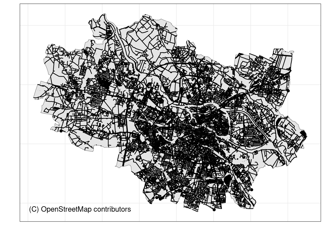
Figure 1 visualizes road networks and the density of it.
References
Footnotes
All signs shared from Wikimedia commons. For similar signs in other European countries have a look on Comparison of European road signs.↩︎
For details see Key:bicycle_road↩︎