Introduction
Looking for a DEM elevation model for entire UK - not in tile form is the query on Open Data StackExchange that prompted this post. The initial question was:
I need to calculate the elevation of 1600 survey plots covering all of the UK - I have these formatted as a point shapefile. I have looked at the OS50 dataset but this is only available as tiles and it would take forever to process each tile individually - my points cover the entire country. Is there free-to-use raster elevation data anywhere that is not split into many tiles?
Let’s review, where to look for Open Source data or what other options we have.
Sources of data for Digital Terrain Models
On the global scale there are few sources available, including:
- SRTM90, SRTM30
- TanDEM-X
NASA held the SRTM (Shuttle Radar Topography Mission) in 2000. The first set of data was released in 2005, however the regions outside the United States were sampled at 3 arc-seconds, which is 1/1200th of a degree of latitude and longitude, or roughly 90 meters on equator (Farr et al. 2007). In 2014 NASA released brand-new dataset with a resolution of 1 arc-second, or roughly 30 meters. Earth Explorer provides the data.
TanDEM-X (TerraSAR-X add-on for Digital Elevation Measurements) data produced by SAR interferometry was acquired in January 2015; the production of the global DEM was completed in September 2016. The absolute height error is with about 1~m. The TanDEM-X 90m DEM publicly available has a pixel spacing of 3 arc-seconds, similar to SRTM90. It covers with 150 Mio sqkm all Earth’s landmasses from pole to pole. More information and data available from EOC Geoservice portal.
For the Europe, there is a set released by Copernicus Programme named EU-DEM v1.0 (or v1.1) — it’s a digital surface model (DSM)1 of European Econemic Area countries. It is a hybrid product based on SRTM and ASTER GDEM data fused by a weighted averaging approach. Detailed description of the dataset and links for download are available under their portal.
All of the above models are characterized by a spatial resolution of 30/90 meters. If more accurate data is needed, look for national sites, where you can download (or buy) the dataset. A few examples:
Czech Republic: You can find (and buy) Digital Terrain Model of the Czech Republic of the 4th (and 5th) generation on Czech Office for Surveying, Mapping and Cadastre (ČÚZK) portal2. As Open Data it provides Data50 set which has been derived from a cartographic database for Base map CR 1 : 50 000 and it is totally comprised of 8 thematic groups. Data are provided as open data in SHP format.
Germany: Federal Agency for Cartography and Geodesy3 provides DEM in 200 m raster (Open Data), however several constituent states provides the data in much better resolution.
Slovakia: Geodesy, Cartography and Cadastre Authority of the Slovak Republic (ÚGKK SR) provides access to DTM data through their portal4 - you can either order the whole set of data or download a small set at once.
Poland: All data available through Head Office of Geodesy and Cartography geoportal.5 DEMs are available as rasters of resolution 1 or 5 m (Open Data).
Raster processing
Let’s acquire and process the data. For raster manipulation we will use terra package (Hijmans 2022), for overall management of spatial features — package sf (Pebesma 2018).
library(terra)
library(sf)
SRTM
To download the SRTM rasters we can use one of elevation_xx() functions from geodata package (Hijmans, Ghosh, and Mandel 2022).
ele <- geodata::elevation_30s("United Kingdom", path = "data")
terra::plot(ele)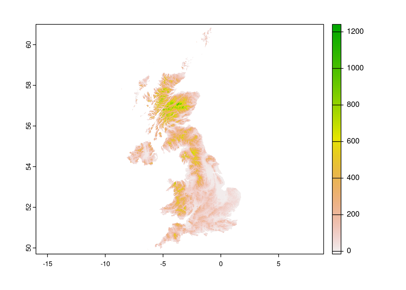
elevation_30s() function returns an aggregated data with spatial resolution about 1 km (30 arc seconds). The data was prepared based on SRTM 90 m and supplemented with the GTOP30 data for latitudes greater than 60 degrees.
Species occurence data
Going back to original question:
I need to calculate the elevation of 1600 survey plots covering all of the UK - I have these formatted as a point shapefile.
Let’s prepare a sample occurrence data for one of the species in UK from GBIF database using rgbif package (Chamberlain, Oldoni, and Waller 2022).
occ <- rgbif::occ_data(
  scientificName = "Calystegia pulchra",
  country = "GB",
  hasCoordinate = TRUE
  )

occ <- head(occ$data, 20) |>
  sf::st_as_sf(coords = c("decimalLongitude", "decimalLatitude"), crs = terra::crs(ele)) |>
  subset(select = c("key", "scientificName"))
Let’s add the observations to the plot:
terra::plot(ele, main = "Sample of C. pulchra distribution in UK")
occ |>
  sf::st_geometry() |>
  plot(add = TRUE)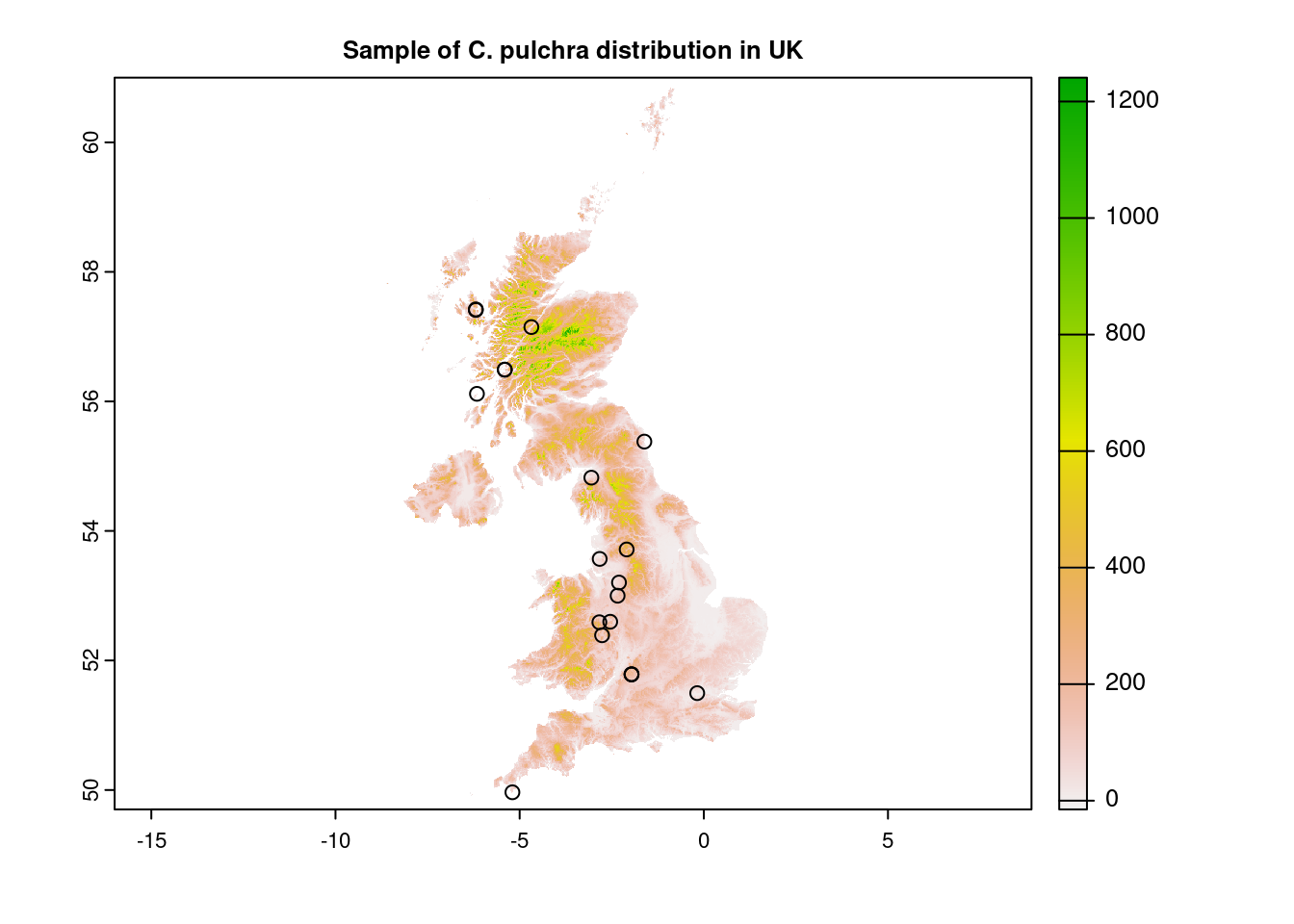
Having our sample data prepared (which is class of sf, tbl_df, tbl, data.frame) we can add the elevation to the set using extract() function form terra. It requires an object of class SpatVector.
occ |>
  dplyr::mutate(elevation = terra::extract(ele, terra::vect(geometry))$GBR_elv_msk) |>
  head(5)
Simple feature collection with 5 features and 3 fields
Geometry type: POINT
Dimension: XY
Bounding box: xmin: -6.189535 ymin: 51.49552 xmax: -0.17902 ymax: 57.41207
Geodetic CRS: WGS 84
# A tibble: 5 × 4
key scientificName geometry elevation
<chr> <chr> <POINT [°]> <dbl>
1 3320924569 Calystegia pulchra Brumm. & Heyw… (-0.17902 51.49553) 16
2 3437494613 Calystegia pulchra Brumm. & Heyw… (-1.962333 51.78564) 209
3 3785877810 Calystegia pulchra Brumm. & Heyw… (-2.541045 52.5979) 186
4 3352641836 Calystegia pulchra Brumm. & Heyw… (-6.189535 57.41207) NaN
5 3338086543 Calystegia pulchra Brumm. & Heyw… (-2.302697 53.20301) 76Points with no value (elevation = NaN) may be caused by inaccuracy or rounding of coordinates when data is normalized by GBIF. In fact, if we checked the fourth point, it would turn out to be at sea. All other elevations are given in meters.
Let’s try more accurate data for UK with 3 arcs sec resolution. Function elevation_3s(lon, lat, ...) from geodata will help to acquire all necessary tiles. To get the lon and lat parameters we will download the UK boundaries and check the bounding box.
uk <- geodata::gadm("United Kingdom", path = "data") |>
  terra::project(terra::crs(ele))

bbox <- sf::st_bbox(uk)
bbox
xmin ymin xmax ymax
-8.649996 49.865310 1.764393 60.845480 for (x in floor(bbox[1]):ceiling(bbox[3])) {
for (y in floor(bbox[2]):ceiling(bbox[4])) {
geodata::elevation_3s(lon = x, lat = y, path = "data")
}
}Error in geodata::elevation_3s(lon = x, lat = y, path = "data"): lat >= -60 & lat <= 60 is not TRUEHmm… In fact the boundary of UK exceeds the 60° N, so, let’s modify our loop (we sacrificed the Shetland Islands, sorry):
for (x in floor(bbox[1]):ceiling(bbox[3])) {
  for (y in floor(bbox[2]):60) {
    geodata::elevation_3s(lon = x, lat = y, path = "data")
  }
}
Having all files downloaded we can build an virtual raster and work with it:
r <- list.files(path = "data", pattern = "srtm_.+.tif", full.names = TRUE)
vrt <- terra::vrt(r, "data/vrt.vrt", overwrite = TRUE) |>
  crop(uk) |>
  mask(uk)
terra::plot(vrt)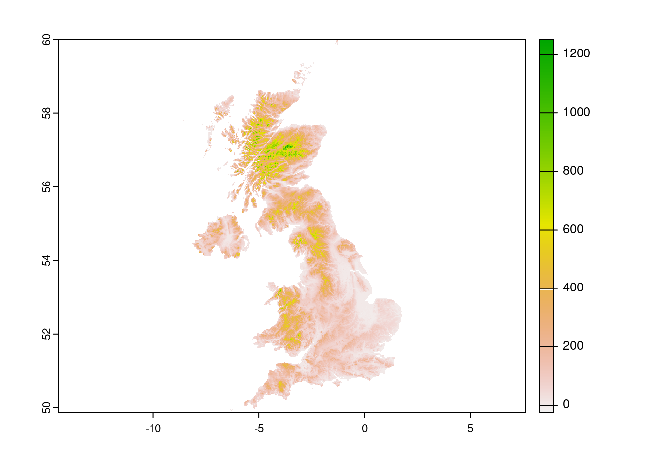
Let’s extract the elevation from our more accurate rasters:
occ |>
  dplyr::mutate(ele_30s = terra::extract(ele, terra::vect(geometry))$GBR_elv_msk) |>
  dplyr::mutate(ele_3s = terra::extract(vrt, terra::vect(geometry))$vrt) |>
  head(5)
Simple feature collection with 5 features and 4 fields
Geometry type: POINT
Dimension: XY
Bounding box: xmin: -6.189535 ymin: 51.49552 xmax: -0.17902 ymax: 57.41207
Geodetic CRS: WGS 84
# A tibble: 5 × 5
key scientificName geometry ele_30s ele_3s
<chr> <chr> <POINT [°]> <dbl> <dbl>
1 3320924569 Calystegia pulchra Brumm.… (-0.17902 51.49553) 16 15
2 3437494613 Calystegia pulchra Brumm.… (-1.962333 51.78564) 209 210
3 3785877810 Calystegia pulchra Brumm.… (-2.541045 52.5979) 186 162
4 3352641836 Calystegia pulchra Brumm.… (-6.189535 57.41207) NaN NA
5 3338086543 Calystegia pulchra Brumm.… (-2.302697 53.20301) 76 73We got quite similar results regardless of resolution. On the other hand, if the your plots are located in mountainous region — the higher the raster resolution, the better.
TanDEM-X
TanDEM data is available from https://download.geoservice.dlr.de/TDM90/ service. To download the necessary data we will use TanDEM package (Simon 2020) available on GitHub.
Please remember to set up the keyring with your user name, like:
keyring::key_set(service = "geoservice.dlr", username = "grzegorz@sapijaszko.net")if(!dir.exists("data/tandem")) { dir.create("data/tandem") }
TanDEM::download_TanDEM(
lon = c(bbox[1], bbox[3]),
lat = c(bbox[2], bbox[4]),
usr = "grzegorz@sapijaszko.net",
srv = "geoservice.dlr",
dstdir = "data/tandem"
)In next step we will build virtual raster and assign NA for cells with no data:
r <- list.files(path = "data/tandem/", pattern = "TDM1_.+.tif", full.names = TRUE)
tandem <- terra::vrt(r, "data/tandem/vrt.vrt", overwrite = TRUE)

terra::NAflag(tandem) <- -32767
Finally, we can extract elevations:
occ |>
  dplyr::mutate(ele_tandem = terra::extract(tandem, terra::vect(geometry))$vrt) |>
  head(5)
Simple feature collection with 5 features and 3 fields
Geometry type: POINT
Dimension: XY
Bounding box: xmin: -6.189535 ymin: 51.49552 xmax: -0.17902 ymax: 57.41207
Geodetic CRS: WGS 84
# A tibble: 5 × 4
key scientificName geometry ele_tandem
<chr> <chr> <POINT [°]> <dbl>
1 3320924569 Calystegia pulchra Brumm. & Heyw… (-0.17902 51.49553) 53.8
2 3437494613 Calystegia pulchra Brumm. & Heyw… (-1.962333 51.78564) 260.
3 3785877810 Calystegia pulchra Brumm. & Heyw… (-2.541045 52.5979) 212.
4 3352641836 Calystegia pulchra Brumm. & Heyw… (-6.189535 57.41207) 57.9
5 3338086543 Calystegia pulchra Brumm. & Heyw… (-2.302697 53.20301) 118. Copernicus data
The original EU-DEM v1.0 (or v1.1) data can be accessed from copernicus.eu portal. It’s divided in 10x10 degree tiles, which results in quite huge files (up to 5 GB per tile). The similar data set, in smaller tiles is available from AWS Opendata Registry. Details in readme. This set can be downloaded by CopernicusDEM package (Mouselimis 2022). Please note, that this dataset is a Digital Surface Model, where elevation measurements represent the surface of the Earth including buildings and infrastructure.
library(CopernicusDEM)

polygon <- sf::st_as_sf(uk)
sf::sf_use_s2(use_s2 = FALSE)

if(!dir.exists("data/copernicus")) { dir.create("data/copernicus")}

aoi_geom_save_tif_matches(
  sf_or_file = polygon,
  dir_save_tifs = "data/copernicus",
  resolution = 30,
  crs_value = 4326,
  threads = parallel::detectCores(),
  verbose = TRUE
)
r <- list.files(path = "data/copernicus/", pattern = "Copernicus_.+.tif", full.names = TRUE)
cop <- terra::vrt(r, "data/copernicus/vrt.vrt", overwrite = TRUE)
occ |>
dplyr::mutate(ele_cop = terra::extract(cop, terra::vect(geometry))$vrt) |>
head(5)Simple feature collection with 5 features and 3 fields
Geometry type: POINT
Dimension: XY
Bounding box: xmin: -6.189535 ymin: 51.49552 xmax: -0.17902 ymax: 57.41207
Geodetic CRS: WGS 84
# A tibble: 5 × 4
key scientificName geometry ele_cop
<chr> <chr> <POINT [°]> <dbl>
1 3320924569 Calystegia pulchra Brumm. & Heyw… (-0.17902 51.49553) 9.39
2 3437494613 Calystegia pulchra Brumm. & Heyw… (-1.962333 51.78564) 218.
3 3785877810 Calystegia pulchra Brumm. & Heyw… (-2.541045 52.5979) 157.
4 3352641836 Calystegia pulchra Brumm. & Heyw… (-6.189535 57.41207) 0
5 3338086543 Calystegia pulchra Brumm. & Heyw… (-2.302697 53.20301) 70.0 ElevatR - the black horse
As the name suggests, elevatr is a package (Hollister 2022) to access elevation data from various sources. With help of get_elev_point() function obtaining the elevation is as simple as:
occ |>
  dplyr::mutate(ele_aws = elevatr::get_elev_point(geometry, src = "aws")$elevation) |>
  head(5)
Mosaicing & ProjectingNote: Elevation units are in metersSimple feature collection with 5 features and 3 fields
Geometry type: POINT
Dimension: XY
Bounding box: xmin: -6.189535 ymin: 51.49552 xmax: -0.17902 ymax: 57.41207
Geodetic CRS: WGS 84
# A tibble: 5 × 4
key scientificName geometry ele_aws
<chr> <chr> <POINT [°]> <dbl>
1 3320924569 Calystegia pulchra Brumm. & Heyw… (-0.17902 51.49553) 15
2 3437494613 Calystegia pulchra Brumm. & Heyw… (-1.962333 51.78564) 191
3 3785877810 Calystegia pulchra Brumm. & Heyw… (-2.541045 52.5979) 169
4 3352641836 Calystegia pulchra Brumm. & Heyw… (-6.189535 57.41207) 44
5 3338086543 Calystegia pulchra Brumm. & Heyw… (-2.302697 53.20301) 75TBC…
References
Footnotes
Digital Surface Model, not Digital Terrain Model!↩︎