The idea of enhance OSM data with highway width came a long ago.1 But instead of using a ortho-photo my aim was to use airborne LIDAR points for analysis. Airborne LIDAR became freely available in last years in several countries and it’s constantly updated. For example Polish Head Office of Geodesy and Cartography (GUGiK) serves LIDAR data since 2010.
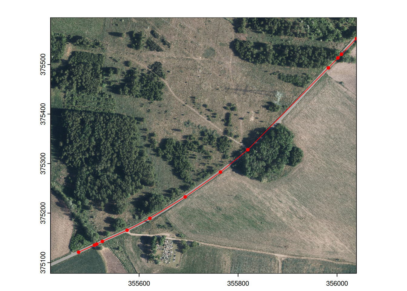
Figure 1: Orthophoto view of the road with vertices added (shown in red).
The approach is to find a point in the middle between pair of vertices and create a 20-m long and 6 m wide “transect” at this point: 10 m left and 10 m right from the road. Figure 2 shows an example.
Figure 2: Analized area of the road: red point – middle of the linestring, green line – perpendicular line with length of 20 m, gray area – analized area: 20x6 m.
Let’s see how LIDAR data looks like in the analyzed area.
The points data contains several classes: ground points, low, middle and high vegetation, etc. We will filter out only points classified as ground and low vegetation. The data is transposed a bit by original buffer bounding box and rotation angle, we have to center it to the linestring mid point.
Figure 4 (a) shows 20 m long crossection of LIDAR points with their height and intensity. You may notice the almost flat area around 0 with uniform intensity which corresponds to the road itself made of asphalt/bituminous mass, the valley on the left and a small bank on the right side of the road. Additional the intensity of ground points is much higher than the road surface itself. We can use those two properties to estimate the width of the road. For that we will take narrow strip (20 cm left, 20 cm right, 40 cm in total) around a mid point, calculate the mean values of height and intensity, their standard deviations and use it as a base values for comparison.
To estimate the road with we will take 10 cm strips starting from -5 to +5 meters in reference to midpoint, calculate the mean values of height and intensity and compare it with base values from the middle. For comparison it was taken (arbitrary): intensity \(I_m\) as \(\bar{I} \pm 2\times\sigma\) and height \(Z_m\) as \(\bar{Z} \pm 3\times\sigma\)
Table 1: Subset of mean intensity (Im) and height (Zm) of (un)classified strips across transects. s – distance from mid point.
s
Im
Zm
road_surface
32
-1.9
37292.50
114.4883
no
33
-1.8
38414.00
114.5200
no
34
-1.7
35513.45
114.4882
yes
35
-1.6
36193.57
114.5271
yes
36
-1.5
35072.78
114.5122
yes
37
-1.4
34678.30
114.5370
yes
38
-1.3
34470.86
114.5257
yes
39
-1.2
33795.55
114.5064
yes
40
-1.1
33959.60
114.5480
yes
41
-1.0
33345.83
114.5375
yes
42
-0.9
33728.14
114.5129
yes
43
-0.8
34486.20
114.5280
yes
44
-0.7
33700.27
114.5200
yes
45
-0.6
33793.75
114.5300
yes
46
-0.5
33878.80
114.5420
yes
47
-0.4
34445.50
114.5117
yes
48
-0.3
35202.70
114.5490
yes
49
-0.2
35038.67
114.5717
yes
50
-0.1
34088.50
114.5330
yes
51
0.0
35361.00
114.5425
yes
52
0.1
34061.73
114.5418
yes
53
0.2
34878.67
114.5444
yes
54
0.3
33752.62
114.5337
yes
55
0.4
33479.00
114.5380
yes
56
0.5
33496.80
114.5490
yes
57
0.6
33835.45
114.5545
yes
58
0.7
33626.33
114.5700
yes
59
0.8
34711.20
114.5360
yes
60
0.9
34230.50
114.5617
yes
61
1.0
34402.89
114.5689
yes
62
1.1
34881.00
114.5411
yes
63
1.2
34808.00
114.5643
yes
64
1.3
35034.22
114.5267
yes
65
1.4
34564.57
114.5771
yes
66
1.5
35080.92
114.5408
yes
67
1.6
34136.00
114.5733
yes
68
1.7
34859.11
114.5456
yes
69
1.8
34938.40
114.5300
yes
70
1.9
35401.08
114.5500
yes
71
2.0
34354.33
114.5183
yes
72
2.1
34154.25
114.5475
yes
73
2.2
34357.40
114.5110
yes
74
2.3
34339.86
114.5429
yes
75
2.4
34822.50
114.5110
yes
76
2.5
34921.38
114.5413
yes
77
2.6
35519.40
114.5130
yes
78
2.7
35043.30
114.5100
yes
79
2.8
35577.00
114.5100
yes
80
2.9
36138.33
114.4900
yes
81
3.0
36402.00
114.5220
yes
82
3.1
35844.50
114.4838
yes
83
3.2
36071.55
114.5064
yes
84
3.3
37230.50
114.4983
no
85
3.4
39068.11
114.5244
no
86
3.5
40422.33
114.5022
no
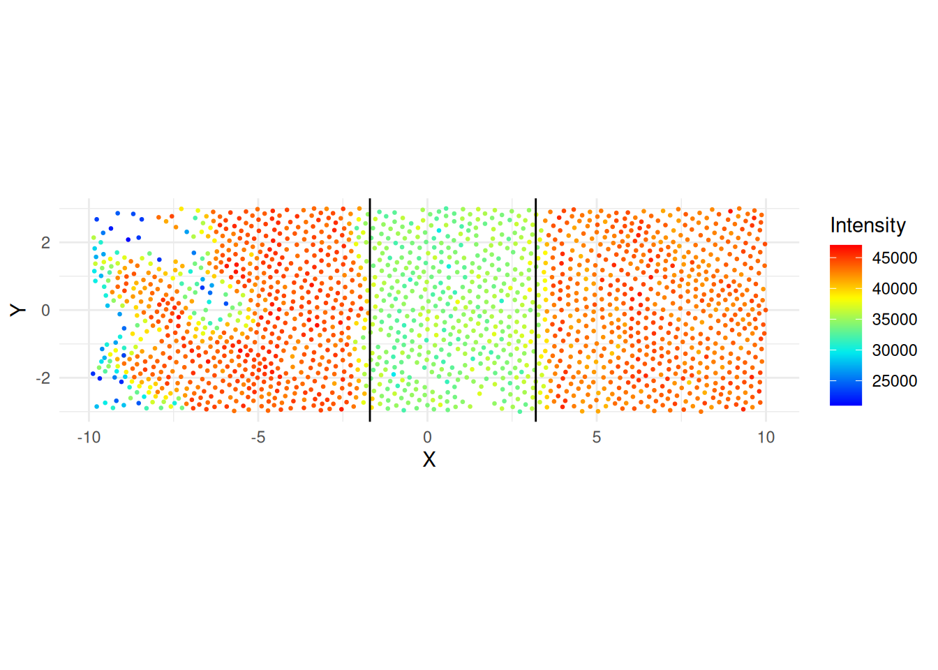
The calculated width is 4.9 meters. Figure 5 shows the LIDAR points with calculated road boundaries. You can notice the shift of the boundaries in the relation to 0 which means that OpenStreetMap line is not drawn centrally to the LIDAR data. The displacement is by 0.75 meters.
Code
ggplot(y@data, aes(X, Y, color = Intensity)) +geom_point(size =0.5) +coord_equal() +theme_minimal() +scale_color_gradientn(colours = lidR::height.colors(50)) +geom_vline(xintercept = h_min) +geom_vline(xintercept = h_max)
Figure 5: LIDAR data plots with road boundaries marked
References
Dyba, Krzysztof, and Jakub Nowosad. 2021. “Rgugik: Search and Retrieve Spatial Data from the Polish Head Office of Geodesy and Cartography in r.”Journal of Open Source Software 6 (59): 2948. https://doi.org/10.21105/joss.02948.
Padgham, Mark, Bob Rudis, Robin Lovelace, Maëlle Salmon, and Joan Maspons. 2023. Osmdata: Import OpenStreetMap Data as Simple Features or Spatial Objects. https://docs.ropensci.org/osmdata/.
Pebesma, Edzer. 2018. “Simple Features for R: Standardized Support for Spatial Vector Data.”The R Journal 10 (1): 439–46. https://doi.org/10.32614/RJ-2018-009.
Roussel, Jean-Romain, and David Auty. 2024. lidR: Airborne LiDAR Data Manipulation and Visualization for Forestry Applications. https://github.com/r-lidar/lidR.
Roussel, Jean-Romain, David Auty, Nicholas C. Coops, Piotr Tompalski, Tristan R. H. Goodbody, Andrew Sánchez Meador, Jean-François Bourdon, Florian de Boissieu, and Alexis Achim. 2020. “lidR: An r Package for Analysis of Airborne Laser Scanning (ALS) Data.”Remote Sensing of Environment 251: 112061. https://doi.org/10.1016/j.rse.2020.112061.
Wickham, Hadley, Winston Chang, Lionel Henry, Thomas Lin Pedersen, Kohske Takahashi, Claus Wilke, Kara Woo, Hiroaki Yutani, Dewey Dunnington, and Teun van den Brand. 2024. Ggplot2: Create Elegant Data Visualisations Using the Grammar of Graphics. https://ggplot2.tidyverse.org.
Footnotes
See Robin’s posts on Mastodon or X. This work started in January 2023, but it was was interrupted by an accident…↩︎