library(osmdata); packageVersion("osmdata")Data (c) OpenStreetMap contributors, ODbL 1.0. https://www.openstreetmap.org/copyright[1] '0.1.10'OpenStreetMap is a project which creates and distributes free geographic data for the world. Based on this data a hundreds of other products evolved, including OSM Map, Nominatim – an open source geocoding service, routing services like OSRM and OpenRouteService among others, several maps styles, etc. For comprehensive overview you can check OSM Wiki.
You can download OpenStreetMap dataset is number of ways1, either the whole planet, a particular region, or ad hock data via Overpass. Build around Overpass API it allows to filter out any feature and get the OSM data quickly. Overpass API is used in osmdata package (Padgham et al. 2017) which will be used in our examples.
Let’s load the library and check it’s version
library(osmdata); packageVersion("osmdata")Data (c) OpenStreetMap contributors, ODbL 1.0. https://www.openstreetmap.org/copyright[1] '0.1.10'OpenStreetMap represents physical features on the Earth using tags attached to its basic data structures (its nodes, ways, and relations). Each tag describes a geographic attribute of the feature being shown by that specific node, way or relation. Those nodes, ways and relations can be translated to geographic objects like points, lines and polygons (closed lines). Relations in OSM are used to describe relationship between features, or other relations. For example Route 662 in US described as relation consist of 11 other relations, which then divides to individual ways. As said, to describe the features a tagging system is used with with key=value pairs, where key corresponds to a topic, category, or type of feature (e.g., highway or name) and value provides detail for the key-specified feature3. A few examples:
boundary = administrative – for any kind of administrative boundaries from hamlet, through community, county to countryamenity = pubhighway = residentialThe typical workflow will follow those steps:
getbb() function)opq())
add_osm_feature() or add_osm_features() for several objects at once)In below example we will get a boundaries of my village, roads, add few amenities and draft it on a map.
Firstly, let’s try to find a bounding box using getbb() function. This function uses Nominatim API to find the bounding box associated with place names.
Lbb <- getbb("Lubnów, Oborniki Śląskie, Poland", format_out = "matrix")
Lbb
min max
x 16.86893 16.90716
y 51.23703 51.28707It may happen, that the result of getbb() slightly differs from expectation. It might be due to misspeling the name, or due the fact, that there is several places with the same name. In such case changing the format_out to data.frame may help.4 Let’s see how many Lubnów’s are in OSM:
getbb("Lubnów", format_out = "data.frame") |>
  select(display_name, boundingbox)
display_name
1 Lubnów, gmina Oborniki Śląskie, powiat trzebnicki, województwo dolnośląskie, Polska
2 Lubnów, gmina Ziębice, powiat ząbkowicki, województwo dolnośląskie, 57-223, Polska
3 Lubnów, gmina Pokój, powiat namysłowski, województwo opolskie, 46-034, Polska
boundingbox
1 51.237034, 51.2870702, 16.868925, 16.9071591
2 50.4920755, 50.5240389, 16.9845096, 17.0430903
3 50.9450812, 50.9850812, 17.8934085, 17.9334085Let’s add a bit of space around. Please remember, the OSM data is provided in EPSG:4326 coordinate system5 (the same used in GPS devices or by Google Maps) where latitude and longitude are given in decimal degrees, so we have to extend the bounding box with the degrees (or tenth of it) as well. We will create a simple matrix and add it to original bbox.
addM <- matrix(data = c(-0.01, -0.01, 0.01, 0.01), nrow = 2, ncol = 2)
newBB <- Lbb + addM
Now, we will create a Overpass query and search for highways using "highway" as a key:
highways <- opq (newBB, timeout = 60) |>
  add_osm_feature (key = "highway") |>
  osmdata_sf()
osmdata_sf returns the data in sf format, which allows smooth integration with sf package. You can use osmdata_sp() for sp format, osmdata_sc() for silicate sc or osmdata_xml() function to get the data in XML format. Let’s grab some other data: administrative boundaries, buildings and a few amenities. We will use add_osm_features() function, which allows to get several features at the time. Features inserted in features = list are combined with logical OR.
otherdata <- opq(newBB, timeout = 60) |>
  add_osm_features(
    features = c(
      "\"boundary\"= \"administrative\"",
      "\"building\"",
      "\"shop\"",
      "\"historic\"=\"archaeological_site\""
    )
  ) |>
osmdata_sf()As the data is already fetched, let’s show them. For visualization we can use just internal plot() function or any fancy package like ggplot2 or osmplotr (Padgham and Beare 2021) which is companion package to osmdata.
Data (c) OpenStreetMap contributors, ODbL 1.0. http://www.openstreetmap.org/copyrightThe data returned from Overpass consist of osm_points, osm_lines, osm_polygons and osm_multipolygons. First of all we have to filter out only those geometries which we will use. Starting with village boundary:
villageBoundary <- otherdata$osm_multipolygons |>
  filter(boundary == "administrative" & admin_level == 8 & name == "Lubnów")
Then splitting roads by its priority, as it will be drawn by lines with different attributes.
secondary <- highways$osm_lines |>
  filter(highway %in% c("secondary"))
tertiary <- highways$osm_lines |>
  filter(highway %in% c("tertiary", "unclassified"))
service <-  highways$osm_lines |>
  filter(highway %in% c("service", "residential"))
track <-  highways$osm_lines |>
  filter(highway %in% c("track"))
And finally buildings, shop(s) and archaeological sites.
buildings <- otherdata$osm_polygons |>
  filter((!is.na(building))) |>
  select(osm_id, geometry)
With shops it will be a bit tricky, as they may appear as a osm_points and/or osm_polygons, where tag shop is assigned to building. We have to ascertain both sets and glue the interesting data together. Another step which will be taken is to find centroids of the polygons and convert it to point geometries, using st_centroid() function from sf package.
shops <- otherdata$osm_points |>
  filter(!is.na(shop)) |>
  select(osm_id, opening_hours, shop, geometry)

shops<- rbind(shops,
      otherdata$osm_polygons |>
        filter(!is.na(shop)) |>
        mutate(geometry = st_centroid(geometry)) |>
        select(osm_id, opening_hours, shop, geometry)
     )
shops <- shops |>
  filter(shop %in% c("convenience", "supermarket"))
And two historical settlements in the neighborhood.
archaeological <- otherdata$osm_points |>
  filter(historic == "archaeological_site") |>
  select(osm_id, historic, geometry)
Let’s build the map using osm_basemap() which set up the boundaries, and then adding features with add_osm_objects() function:
map <- osm_basemap(bbox = newBB, bg = "gray95")
map <- add_osm_objects(map, villageBoundary, col = "gray99", border = "red", size = 1.2)
map <- add_osm_objects(map, secondary, size = 3, shape = 1, col = "orange")
map <- add_osm_objects(map, secondary, size = 1.2, shape = 1, col = "darkred")
map <- add_osm_objects(map, tertiary, col = "black", size = 0.8)
map <- add_osm_objects(map, service, col = "gray40", size = 0.4)
map <- add_osm_objects(map, track, col = "gray60", size = 0.2)
map <- add_osm_objects(map, buildings, col = "brown")
map <- add_osm_objects(map, shops, size = 3, col = "darkblue")
map <- add_osm_objects(map, archaeological, size = 3, col = "darkgreen")
map <- add_axes (map, colour = "blue", pos = c(0.02, 0.02),
          fontsize = 4, fontface = 2, fontfamily = "Times")
And finally let’s print the map:
print_osm_map(map)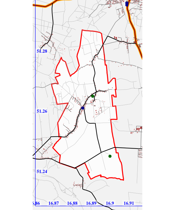
for details see https://wiki.openstreetmap.org/wiki/Downloading_data↩︎
https://www.openstreetmap.org/relation/93155↩︎
For comprehensive list see https://wiki.openstreetmap.org/wiki/Map_features↩︎
Instead of matrix or data.frame we can get the result of getbb() as polygon or sf_polygon for polygons that work with sf package.↩︎
https://epsg.io/4326↩︎